Standard Error calculation on EMB verification pages
The estimate of verification metrics at each forecast length has an associated uncertainty due, in part, to the small number of runs going into the sample.
For profile plots, dieoff plots, diurnal plots, and time series plots with temporal averaging, we don’t see the statistics from the underlying individual runs (although they can be seen on
the time series page if no averaging is used), but we can estimate the uncertainty in the mean statistic by considering the variations in the statistic over the time series of the matched model runs in the sample. The uncertainty of the mean (“standard error”) is estimated as:
Standard Error = σ/sqrt[(n-1)(1-φ)]
where σ is the standard deviation, n is the number of values in the sample, x is the
set of statistics, and φ Is the lag one autocorrelation derived from the time series x. This is
empirically derived from the individual values with the approximation:
φ ≅ cor(x_(1 … (n - 1)),x_(x … n))
The estimate of the standard error on the mean is distinct and separate from the
standard deviation from the sample. The standard error is an estimate of how well we
understand the underlying, fundamental statistic at each forecast length. The standard
deviation is an estimate of how far off the mean value any one statistic may be
(Weatherhead et al., 1998). Thus, were our sample of runs to be repeated in a similar
season and for a similar duration, we can say that the mean statistic has a 67% likelihood of
being within one standard error of our results, and a 95% likelihood of being within two (1.96)
standard errors of our results.
This approach at least partially accommodates the fact that the individual statistics are autocorrelated.
Physically, this implies that weather situations, which can be more or less forecastable, can last for more than one day, thus the sequential forecast statistics are not independent estimates, but represent an over-sampling of the system. The standard error equation above accounts for these. It should be noted that the lag 1 AutoRegressive assumption generally refers to a 12-hour lag (for runs that are verified every 12 h) or 24-hour lag (for 00Z or 12Z only verification) as the most significant approximation to the autocorrelation. It should also be noted that aggregation of 00Z and 12Z results allows for a larger sample size, but may result in combining different physical causes of differences as well as different statistical properties of the time series.
We generate the errors on the paired differences in the same way. That is, for each forecast
length, we generate a time series of paired differences, and calculate the mean and
standard error for the differences using the methods described above.
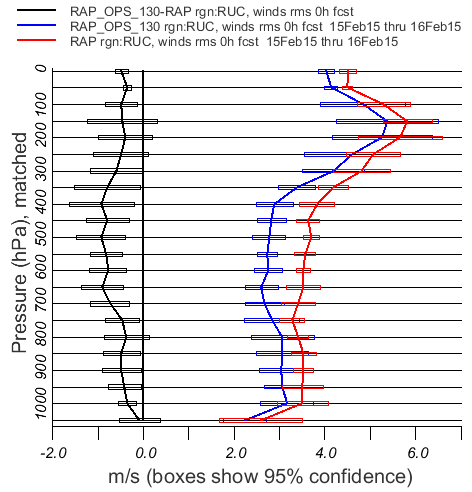
In the figures generated, the boxes indicate +/- 2 (actually 1.96) standard errors from the mean. If, for instance, a difference curve is one half-box away from the zero line, that difference is statistically significant at the 95% confidence level.
As an example, the figure below shows a difference curve that is significantly (95%) different from zero at most altitudes, but not at 150, 800, 300-150 hPa.
Also, in the figure below the situation at 1000 hPa shows the power of paired differences: The errors on the red and blue curves at 1000 nPa overlap considerably, suggesting that the difference in the overall vector wind RMSE for the period are not significant (at the 95% confidence level). But the difference curve which represents the statistical mean and standard error of the time-matched paired differences is significantly different from zero.
Some important details:
Reference:
Weatherhead, E. C., G. C. Reinsel, G. C. Tiao, X. Meng, D. Choi, W. Cheang, T. Keller,
J. DeLuisi, D. J. Wuebbles, J. B. Kerr, A. J. Miller, S. J. Oltmans, and J. E. Frederick,
1998: Factors affecting the detection of trends: Statistical considerations and
applications to environmental data. Journal of Geophysical Research, 103, 17149-
17161.